Building a Schedule Matrix

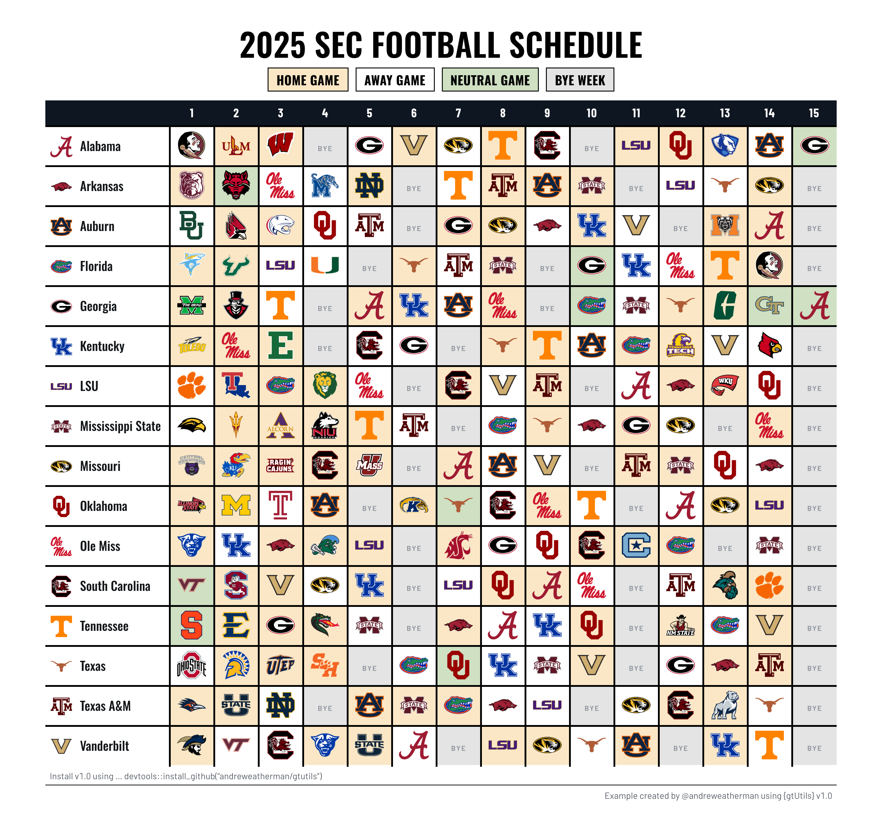
The catch with a schedule matrix is the coloring. You want a cell shaded by whether that game is home, away, or on a neutral field, and a different shade for a bye. That is a decision made cell by cell, not column by column, and it is where a schedule matrix gets awkward to build.

The old approach was to hand-write CSS: loop over row and column indices, build an nth-child selector for every cell that should be shaded, and inject the lot through opt_css(). It works, but it is a lot of machinery for what is really one condition applied to a grid of cells.

v1.0 adds gt_highlight_cells(), which fills individual cells by a condition, and gt_legend_discrete(), which draws the matching key. This vignette builds a full SEC schedule matrix with both, and picks up a few other v1.0 habits along the way.

The data

We pull the 2025 FBS schedule from cfbfastR-data, double it into one row per team with nflreadr::clean_homeaway(), and keep the SEC. clean_homeaway() renames the home_* / away_* pairs to team_* / opponent_* based on where each team played, so the same team_id we use for the opponent’s logo also gives us each team’s own logo.

base <- "http://a.espncdn.com/i/teamlogos/ncaa/500/"

data <- read_csv("https://github.com/sportsdataverse/cfbfastR-data/raw/refs/heads/main/schedules/csv/cfb_schedules_2025.csv") %>%
  filter(season_type == "regular") %>%
  select(home_team, away_team, week, home_conference, away_conference,
         home_id, away_id, neutral_site) %>%
  nflreadr::clean_homeaway() %>%
  filter(team_conference == "SEC") %>%
  mutate(opponent_logo = paste0(base, opponent_id, ".png"),
         team_logo = paste0(base, team_id, ".png"),
         location = ifelse(neutral_site == TRUE, "neutral", location)) %>%
  select(team, team_logo, week, location, opponent_logo)

clean_homeaway() sets location to "home" or "away", so we fold the schedule’s neutral_site flag into that same column as a third value.

logos <- data %>%
  arrange(team) %>%
  pivot_wider(id_cols = c(team, team_logo), names_from = week,
              values_from = opponent_logo, names_sort = TRUE)

wk <- setdiff(names(logos), c("team", "team_logo"))

names_sort = TRUE sorts the week columns. Because week is numeric, they come out 1 through 15 in order rather than 1, 10, 11, .... Carrying team_logo through id_cols keeps each team’s logo alongside its row without a second join.

Carrying the location as a parallel mask

pivot_wider() on the opponent logo loses the location. But we can pivot it into its own frame of the same shape and turn each state into a logical mask.

locs <- data %>% pivot_wider(id_cols = team, names_from = week, values_from = location)
locs <- locs[match(logos$team, locs$team), ]

home_mask <- as.data.frame(locs[, wk] == "home")
away_mask <- as.data.frame(locs[, wk] == "away")
neutral_mask <- as.data.frame(locs[, wk] == "neutral")

The match() line reorders locs to follow logos, so both frames share a row order after the arrange(). Each mask is then a TRUE/FALSE grid the same shape as the week columns, which is what gt_highlight_cells() takes.

Filling cells by condition

gt_highlight_cells() fills the cells in a block of columns that meet a condition. The condition is either a formula tested against each column, like ~ is.na(.x), or a logical matrix the same shape as the columns, which is what our masks are. It is the per-cell counterpart to gtExtras::gt_highlight_cols() and gt_highlight_rows(), which fill whole columns or rows.

gt_highlight_cells(all_of(wk), condition = home_mask, fill = "#FBE7C6") %>%
gt_highlight_cells(all_of(wk), condition = away_mask, fill = "#FFFFFF") %>%
gt_highlight_cells(all_of(wk), neutral_mask, fill = "#CFE0C3") %>%
gt_highlight_cells(all_of(wk), condition = ~ is.na(.x), fill = "#E4E4E4")

Home, away, and neutral come from the masks. The bye is any cell with no game, which is a missing opponent, so ~ is.na(.x) catches it without a mask of its own.

gt_highlight_cells() has more arguments (text_color, bold, and ... to cell_text()) for when you want to style the text as well as the fill.

Drawing the logos

With the cells shaded, we render the opponent URLs as images with gtExtras::gt_img_rows(), one week column at a time.

purrr::reduce(wk, .init = ., .f = ~ rlang::inject(
  gtExtras::gt_img_rows(.x, columns = !!rlang::sym(.y), height = 35)
))

gt_img_rows() takes a single column, and it reads a quoted number like "1" as a position rather than a name, so all_of() fails on our numeric week columns. reduce() threads the table through one call per week, and !!rlang::sym(.y) hands each column in as a bare name, which is the form gt_img_rows() wants. Keeping this inside the pipe means no stored intermediate.

Marking the byes

After the images render, we drop a muted BYE into the empty cells.

byemark <- "<span style=\"color:#8A9099;font-size:8px;font-weight:600;letter-spacing:0.12em\">BYE</span>"

reduce(wk, .init = ., .f = function(g, c) {
  b <- which(is.na(logos[[c]])); if (!length(b)) return(g)
  text_transform(g, cells_body(columns = all_of(c), rows = b), fn = function(x) byemark)
})

This has to run after gt_img_rows(), not through sub_missing(), because gt_img_rows() would otherwise wrap the placeholder text in a broken <img> tag. We find the missing rows per column and write the mark straight into them.

Logo and name in the team column

We can render the team logo and name together in a flex container and pin the column width so a long name wraps instead of stretching the table.

team_cell <- function(name, logo) sprintf(
  '<div style="display:flex; align-items:center; gap:8px;">
     <img src="%s" style="height:26px; width:26px; object-fit:contain; flex:none;">
     <span style="font-family:\'Oswald\',sans-serif; font-size:14px; font-weight:500;
                  line-height:1.05;">%s</span></div>',
  logo, name)

text_transform(cells_body(columns = team),
               fn = \(x) unname(mapply(team_cell, logos$team, logos$team_logo)))

flex:none holds the logo at 26px so the name takes the rest of a fixed column. We map from logos$team and logos$team_logo rather than the x the transform receives, because gt HTML-escapes the cell first, turning, e.g., “Texas A&M” into “Texas A&M”.

The legend

gt_legend_discrete() draws the key, the categorical partner to gt_legend_continuous(). Pass it a named vector of label = color and it renders the swatches, using the same fills as the cells so the key matches the table.

gt_legend_discrete(
  c("Home Game" = "#FBE7C6", "Away Game" = "#FFFFFF",
    "Neutral Game" = "#CFE0C3", "Bye Week" = "#E4E4E4"),
  location = "top", label_placement = "inside", shape = "square",
  gap = 8, swatch_size = 20, border_width = 1.5, border_color = "black",
  heading = "2025 SEC Football Schedule",
  heading_style = list(font = "Oswald", size = 36, weight = 600,
                       transform = "uppercase", margin_bottom = -5),
  label_style = list(font = "Oswald", size = 14, margin_bottom = 6)
)

label_placement = "inside" prints each label on its swatch, and the text color is chosen per-swatch for contrast. The heading_style and label_style lists follow the same convention as gt_grid() and gt_title_header(): font, size, color, weight, italic, spacing, transform, and align, plus line_height and the margin_* and padding_* keys. margin_bottom = -5 pulls the key up tight under the title.

Putting it together

The whole pipeline, from the wide frame to the finished image:

gt(logos, id = "table") %>%
  gt_theme_scoreboard() %>%
  cols_hide(team_logo) %>%
  gt_highlight_cells(all_of(wk), condition = home_mask, fill = "#FBE7C6") %>%
  gt_highlight_cells(all_of(wk), condition = away_mask, fill = "#FFFFFF") %>%
  gt_highlight_cells(all_of(wk), neutral_mask, fill = "#CFE0C3") %>%
  gt_highlight_cells(all_of(wk), condition = ~ is.na(.x), fill = "#E4E4E4") %>%
  purrr::reduce(wk, .init = ., .f = ~ rlang::inject(
    gtExtras::gt_img_rows(.x, columns = !!rlang::sym(.y), height = 35)
  )) %>%
  reduce(wk, .init = ., .f = function(g, c) {
    b <- which(is.na(logos[[c]])); if (!length(b)) return(g)
    text_transform(g, cells_body(columns = all_of(c), rows = b), fn = function(x) byemark)
  }) %>%
  text_transform(cells_body(columns = team),
                 fn = \(x) unname(mapply(team_cell, logos$team, logos$team_logo))) %>%
  cols_align(columns = -team, "center") %>%
  gt_border_grid(weight = 2) %>%
  tab_options(table_body.hlines.width = px(2)) %>%
  cols_width(-team ~ px(50), team ~ px(140)) %>%
  cols_label(team = "") %>%
  tab_style(locations = cells_column_labels(), cell_text(size = px(14))) %>%
  gt_legend_discrete(
    c("Home Game" = "#FBE7C6", "Away Game" = "#FFFFFF",
      "Neutral Game" = "#CFE0C3", "Bye Week" = "#E4E4E4"),
    location = "top", label_placement = "inside", shape = "square",
    gap = 8, swatch_size = 20, border_width = 1.5, border_color = "black",
    heading = "2025 SEC Football Schedule",
    heading_style = list(font = "Oswald", size = 36, weight = 600,
                         transform = "uppercase", margin_bottom = -5),
    label_style = list(font = "Oswald", size = 14, margin_bottom = 6)) %>%
  gt_538_caption(
    md('Install v1.0 using ... devtools::install_github("andreweatherman/gtutils")'),
    "Example created by @andreweatherman using {gtUtils} v1.0")